Generally speaking, one should keep pipeline steps as simple as possible, basically following the principle “one step, one task”. While splitting up analysis steps into multiple functions naturally becomes hard to manage with a growing number of functions, with {pipeflow}, which manages all function and parameter dependencies for you, this feels rather easy.
Following this principle, most of the pipeline steps will carry intermediate results while only a few steps contain the final output we are interested in.
This vignette shows how to conveniently tag and collect those final outputs as well as how to filter pipelines via {pipeflow}s view functionality.
Tagging steps
Tags let you label steps with meaningful keywords so you can later
filter the pipeline by topic, stage, or output type. Tags can be set
during pipeline creation or later using pip_set_tags().
library(pipeflow)

pip <- pip_new("my-pip") |>
    pip_add(
        "data",
        function(data = airquality) data
    ) |>
    pip_add("data_prep",
        function(data = ~data) {
            replace(data, "Temp.Celsius", (data[, "Temp"] - 32) * 5 / 9)
        },
        tags = "data"                   # <-- set 'data' tag
    ) |>
    pip_add(
        "data_summary",
        function(
            data = ~data_prep,
            xVar = "Temp.Celsius",
            yVar = "Ozone"
        ) {
            format(summary(data[, c(xVar, yVar)])) |>
                as.data.frame(row.names = NA)
        },
        tags = c("data", "summary")     # <-- set 'data' and 'summary' tags
    ) |>
    pip_add(
        "data_plot",
        function(
            data = ~data_prep,
            xVar = "Temp.Celsius",
            yVar = "Ozone"
        ) {
            require(ggplot2, quietly = TRUE)
            ggplot(data) +
                geom_point(aes(.data[[xVar]], .data[[yVar]])) +
                labs(title = "Data")
        },
        tags = c("data", "plot")        # <-- set 'data' and 'plot' tags
    ) |>
    pip_add(
        "model_fit",
        function(
            data = ~data_prep,
            xVar = "Temp.Celsius",
            yVar = "Ozone"
        ) {
            lm(paste(yVar, "~", xVar), data = data)
        },
        tags = c("model", "fit")        # <-- set 'model' and 'fit' tags
    ) |>
    pip_add(
        "model_summary",
        function(fit = ~model_fit) {
            summary(fit) |>
                coefficients() |>
                as.data.frame()
        },
        tags = c("model", "summary")    # <-- set 'model' and 'summary' tags
    ) |>
    pip_add(
        "model_plot",
        function(
            model = ~model_fit,
            data_plot = ~data_plot,
            xVar = "Temp.Celsius",
            yVar = "Ozone"
        ) {
            coeffs <- coefficients(model)
            data_plot +
                geom_abline(intercept = coeffs[1], slope = coeffs[2]) +
                labs(title = "Linear model fit")
        },
        tags = c("model", "plot")       # <-- set 'model' and 'plot' tags
    )
We used two families of tags:
"data"/"model" to distinguish the topic, and
"summary"/"plot"/"fit" for the
output type. Whenever tags are defined, they are shown in the pipeline
overview (see rightmost column):
pip
# <pipeflow_pip> my-pip (7 steps)
# -------------------------------
#             step             depends    out state          tags
# 1:          data                     [NULL]   new
# 2:     data_prep                data [NULL]   new          data
# 3:  data_summary           data_prep [NULL]   new  data,summary
# 4:     data_plot           data_prep [NULL]   new     data,plot
# 5:     model_fit           data_prep [NULL]   new     model,fit
# 6: model_summary           model_fit [NULL]   new model,summary
# 7:    model_plot model_fit,data_plot [NULL]   new    model,plot
Before showing how to make use of the tags, let’s run the pipeline and inspect the output individually as we did in the previous vignettes.
pip_run(pip)
# info [2026-06-27 18:20:44.042 UTC]: Start run of pipeflow_pip 'my-pip'
# info [2026-06-27 18:20:44.043 UTC]: Step 1/7 data
# info [2026-06-27 18:20:44.045 UTC]: Step 2/7 data_prep
# info [2026-06-27 18:20:44.048 UTC]: Step 3/7 data_summary
# info [2026-06-27 18:20:44.051 UTC]: Step 4/7 data_plot
# info [2026-06-27 18:20:44.794 UTC]: Step 5/7 model_fit
# info [2026-06-27 18:20:44.801 UTC]: Step 6/7 model_summary
# info [2026-06-27 18:20:44.810 UTC]: Step 7/7 model_plot
# info [2026-06-27 18:20:44.816 UTC]: Finished run of pipeflow_pip 'my-pip'

pip
# <pipeflow_pip> my-pip (7 steps)
# -------------------------------
#             step             depends                 out state          tags
# 1:          data                     <data.frame[153x6]>  done
# 2:     data_prep                data <data.frame[153x7]>  done          data
# 3:  data_summary           data_prep   <data.frame[7x2]>  done  data,summary
# 4:     data_plot           data_prep   <ggplot2::ggplot>  done     data,plot
# 5:     model_fit           data_prep            <lm[13]>  done     model,fit
# 6: model_summary           model_fit   <data.frame[2x4]>  done model,summary
# 7:    model_plot model_fit,data_plot   <ggplot2::ggplot>  done    model,plot
pip[["data_plot", "out"]]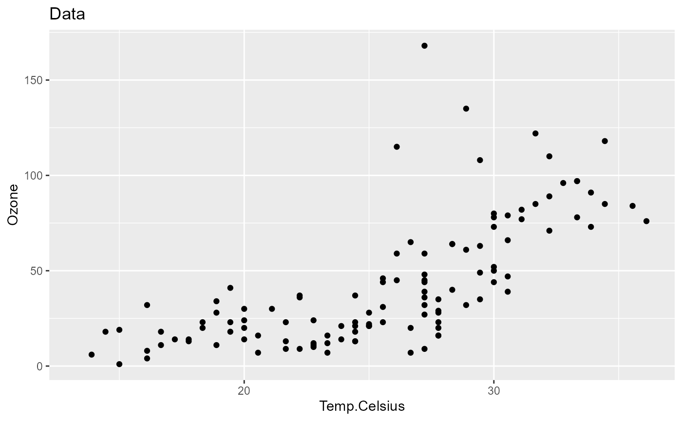
pip[["model_plot", "out"]]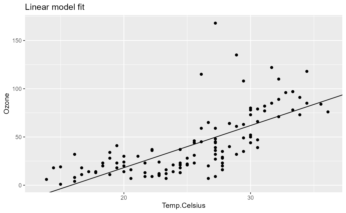
Flat output collection
pip_collect_out() returns all step outputs as a flat
named list1.
out <- pip_collect_out(pip)

names(out)
# [1] "data"          "data_prep"     "data_summary"  "data_plot"     "model_fit"     "model_summary"
# [7] "model_plot"
Filtered output using tags
To collect only the output of steps with a specific tag, we use
pip_view(), which is {pipeflow}’s general-purpose function
for filtering pipelines, and then call pip_collect_out() on
the filtered pipeline view. For example, to collect only the plots, we
can filter by the plot tag.
pip_view(pip, tags = "plot")
# <pipeflow_view> my-pip view (2 of 7 steps)
# ------------------------------------------
#        step             depends               out state       tags
#   data_plot           data_prep <ggplot2::ggplot>  done  data,plot
#  model_plot model_fit,data_plot <ggplot2::ggplot>  done model,plot
pip |>
    pip_view(tags = "plot") |>
    pip_collect_out() |>
    gridExtra::grid.arrange(grobs = _, nrow = 2)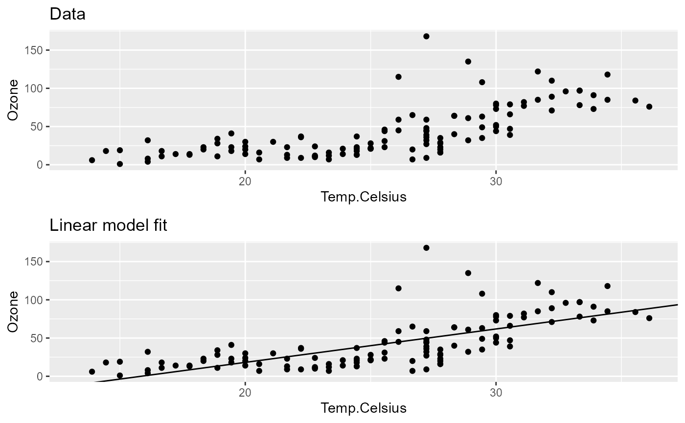
Grouped output via views
Grouped output is achieved by composing pip_view() with
pip_collect_out(). For example, to collect outputs grouped
by topic ("data" and "model"):
grouped <- list(
    data  = pip_view(pip, tags = "data")  |> pip_collect_out(),
    model = pip_view(pip, tags = "model") |> pip_collect_out()
)

names(grouped[["data"]])
# [1] "data_prep"    "data_summary" "data_plot"
names(grouped[["model"]])
# [1] "model_fit"     "model_summary" "model_plot"
More on views
To make the example a bit more interesting, we first update some parameters.
pip_set_params(pip, params = list(xVar = "Solar.R", yVar = "Wind"))

pip
# <pipeflow_pip> my-pip (7 steps)
# -------------------------------
#             step             depends                 out    state          tags
# 1:          data                     <data.frame[153x6]>     done
# 2:     data_prep                data <data.frame[153x7]>     done          data
# 3:  data_summary           data_prep   <data.frame[7x2]> outdated  data,summary
# 4:     data_plot           data_prep   <ggplot2::ggplot> outdated     data,plot
# 5:     model_fit           data_prep            <lm[13]> outdated     model,fit
# 6: model_summary           model_fit   <data.frame[2x4]> outdated model,summary
# 7:    model_plot model_fit,data_plot   <ggplot2::ggplot> outdated    model,plot
{pipeflow} views provide a variety of filtering options. In the
previous section, the filtering was done based on tags, but you can also
filter based on other properties, for example, to select all
outdated steps that depend on the model_fit
step:
pip |> pip_view(filter = list(depends = "model_fit", state = "outdated"))
# <pipeflow_view> my-pip view (2 of 7 steps)
# ------------------------------------------
#           step             depends               out    state          tags
#  model_summary           model_fit <data.frame[2x4]> outdated model,summary
#     model_plot model_fit,data_plot <ggplot2::ggplot> outdated    model,plot
or using regex-based filtering to filter all outdated steps starting
with data:
pip |>
    pip_view(filter = list(step = "^data", state = "outdated"), fixed = FALSE)
# <pipeflow_view> my-pip view (2 of 7 steps)
# ------------------------------------------
#          step   depends               out    state         tags
#  data_summary data_prep <data.frame[7x2]> outdated data,summary
#     data_plot data_prep <ggplot2::ggplot> outdated    data,plot
Views can also be chained together:
v <- pip |> pip_view(filter = list(state = "outdated"))
v
# <pipeflow_view> my-pip view (5 of 7 steps)
# ------------------------------------------
#           step             depends               out    state          tags
#   data_summary           data_prep <data.frame[7x2]> outdated  data,summary
#      data_plot           data_prep <ggplot2::ggplot> outdated     data,plot
#      model_fit           data_prep          <lm[13]> outdated     model,fit
#  model_summary           model_fit <data.frame[2x4]> outdated model,summary
#     model_plot model_fit,data_plot <ggplot2::ggplot> outdated    model,plot

v2 <- v |> pip_view(tags = "plot")
v2
# <pipeflow_view> my-pip view view (2 of 7 steps)
# -----------------------------------------------
#        step             depends               out    state       tags
#   data_plot           data_prep <ggplot2::ggplot> outdated  data,plot
#  model_plot model_fit,data_plot <ggplot2::ggplot> outdated model,plot
Last but not least, views can be run as pipelines themselves, which allows to conveniently re-run only the filtered steps, while {pipeflow} ensures that any upstream dependencies are run first if needed.
v2 |> pip_run()
# info [2026-06-27 18:20:46.931 UTC]: Start run of pipeflow_view 'my-pip view view'
# info [2026-06-27 18:20:46.931 UTC]: Step 1/4 [upstream] data_prep - skipping done step
# info [2026-06-27 18:20:46.932 UTC]: Step 2/4 [view] data_plot
# info [2026-06-27 18:20:46.951 UTC]: Step 3/4 [upstream] model_fit
# info [2026-06-27 18:20:46.955 UTC]: Step 4/4 [view] model_plot
# info [2026-06-27 18:20:46.965 UTC]: Finished run of pipeflow_view 'my-pip view view'
Having a closer look at the run log, you’ll see which steps were
re-run as part of the [view] and which were re-run as
[upstream] dependencies. Since all views work by reference
on the given pipeline, the original pipeline is now up-to-date for the
filtered steps.
pip
# <pipeflow_pip> my-pip (7 steps)
# -------------------------------
#             step             depends                 out    state          tags
# 1:          data                     <data.frame[153x6]>     done
# 2:     data_prep                data <data.frame[153x7]>     done          data
# 3:  data_summary           data_prep   <data.frame[7x2]> outdated  data,summary
# 4:     data_plot           data_prep   <ggplot2::ggplot>     done     data,plot
# 5:     model_fit           data_prep            <lm[13]>     done     model,fit
# 6: model_summary           model_fit   <data.frame[2x4]> outdated model,summary
# 7:    model_plot model_fit,data_plot   <ggplot2::ggplot>     done    model,plot