Overview
{targets} is the most widely used pipeline toolkit in the R ecosystem and the de-facto standard for heavy-duty reproducible workflows. The table below contrasts the two packages to help you decide which one fits your project.
| Feature | targets | pipeflow |
|---|---|---|
| Paradigm | Declarative — define the full DAG upfront in a
_targets.R script, then execute |
Interactive — incrementally build the pipeline with
pip_add() as you code |
| Execution |
tar_make() runs in a fresh R
process
|
pip_run() runs in the current R
session
|
| Persistent storage | ✅ Output stored to disk (_targets/objects/), survives
R restarts, handles data larger than RAM |
❌ In-memory only, lost when R session ends |
| Skip up-to-date steps | ✅ Hash-based invalidation of code and data | ✅ State-based (done / outdated) |
| Metadata & provenance | ✅ tar_meta() records runtime, size, errors per
target |
❌ No per-step provenance metadata |
| Dependency validation | ✅ tar_validate() for pre-flight checks (opt-in) |
✅ On pip_add(), pip_replace(),
pip_remove() — fails fast on broken references |
| Modify pipeline at runtime | ❌ Must edit _targets.R and re-run |
✅ pip_remove(), pip_rename(),
pip_replace(), insert with after =
|
| Parameter management | ❌ No unified parameter view across targets | ✅ pip_get_params() / pip_set_params() —
one call updates all steps |
| Split / map / reduce | ✅ pattern = map() / cross() built-in,
tarchetypes for advanced patterns |
✅ Built-in exec = "split" / "auto" /
"reduce"
|
| Dynamic branching | ✅ Comprehensive via tarchetypes
|
✅ Auto-mapping over partition keys
(exec = "auto") |
| Views / tag filtering |
tar_described_as() selects by description tags |
✅ pip_view() — filter steps by tags or index |
| Pipeline composition | ❌ | ✅ pip_bind() two pipelines,
pip_add_from() copy individual steps |
| Self-modifying pipelines | ❌ | ✅ pip_run(recursive = TRUE) — steps can return
modified pipelines |
| Distributed computing | ✅ crew for HPC and cloud workers |
❌ |
| Cloud storage | ✅ AWS, GCS | ❌ |
| File tracking | ✅ File targets with format = "file"
|
❌ |
| Step locking | ❌ | ✅ pip_lock() / pip_unlock() — protect
steps from accidental modification |
In short, {targets} is the tool of choice for
large-scale reproducible projects: it persists results to disk, captures
provenance with tar_meta(), and scales to distributed
infrastructure via crew. {pipeflow}
prioritises speed and interactivity — sub-millisecond skipped-step
checks, in-session pipeline modification, and low response times make it
well suited as a Shiny backend or for rapid parameter exploration during
analysis.
Benchmarks
The benchmarks below provide a quantitative comparison on three
pipeline topologies. All timings are measured with
system.time() across 30 iterations per scenario.
Package versions: pipeflow 0.3.0, targets 1.12.0.
The three scenarios were chosen to isolate different aspects of pipeline overhead:
- Walkthrough — a minimal 4-step pipeline mimicking a typical exploratory workflow. This measures startup cost and skip-check overhead in the simplest realistic case.
-
Long linear pipeline — a chain of N steps
(
s0 -> s1 -> ... -> sN). This isolates per-step bookkeeping cost as the pipeline grows to 128 steps. - Fan-out DAG — a single source feeds N parallel branches that converge on one sink. This tests how each package handles wide dependency structures.
For targets, each iteration uses a fresh tar_dir() and
tar_script() to ensure fair timing of end-to-end pipeline
execution. For pipeflow, pipelines are built once and timed with
force = TRUE to measure the cost of a full re-run.
Walkthrough example
A minimal four-step pipeline based on the {targets}
walkthrough — read CSV data, fit a linear model, and produce a plot.
We measure both the first full run (all steps executed) and the
subsequent skipped run (all steps already up to date). Full runs with
targets include a tar_destroy() between iterations so each
is a true cold start.
create_data_csv <- function(data = airquality, file = "data.csv") {
    utils::write.csv(data, file)
}

get_data <- function(file) {
    utils::read.csv(file) |> stats::na.omit()
}

fit_model <- function(data) {
    lm(Ozone ~ Temp, data) |> coefficients()
}

plot_model <- function(model, data) {
    ggplot(data) +
        geom_point(aes(x = Temp, y = Ozone)) +
        geom_abline(intercept = model[1], slope = model[2])
}
pipeflow pipeline
tar_dir({
    create_data_csv(file = "data.csv")
    p <- pip_new("walkthrough") |>
        pip_add("data",  \(file = "data.csv") get_data(file)) |>
        pip_add("model", \(data = ~data) fit_model(data)) |>
        pip_add(
            "plot",
            \(model = ~model, data = ~data) plot_model(model, data)
        )

    message("\nProof of principle full run (no skips)")
    pip_run(p)
    p_r <- replicate(nrep, elapsed_time(pip_run(p, lgr = NULL, force = TRUE)))

    message("\nProof of principle skipped run")
    pip_run(p)
    p_s <- replicate(nrep, elapsed_time(pip_run(p, lgr = NULL)))
})
#
# Proof of principle full run (no skips)
# info [2026-06-20 19:20:51.077 UTC]: Start run of pipeflow_pip 'walkthrough'
# info [2026-06-20 19:20:51.077 UTC]: Step 1/3 data
# info [2026-06-20 19:20:51.083 UTC]: Step 2/3 model
# info [2026-06-20 19:20:51.089 UTC]: Step 3/3 plot
# info [2026-06-20 19:20:51.121 UTC]: Finished run of pipeflow_pip 'walkthrough'
#
# Proof of principle skipped run
# info [2026-06-20 19:20:51.560 UTC]: Start run of pipeflow_pip 'walkthrough'
# info [2026-06-20 19:20:51.560 UTC]: Step 1/3 data - skipping done step
# info [2026-06-20 19:20:51.560 UTC]: Step 2/3 model - skipping done step
# info [2026-06-20 19:20:51.560 UTC]: Step 3/3 plot - skipping done step
# info [2026-06-20 19:20:51.561 UTC]: Finished run of pipeflow_pip 'walkthrough'
targets pipeline
tar_make_here <- function(reporter = "silent") {
    tar_make(callr_function = NULL, reporter = reporter)
}

tar_dir({
    create_data_csv(file = "data.csv")
    tar_script({
        list(
            tar_target(file, "data.csv", format = "file"),
            tar_target(data, get_data(file)),
            tar_target(model, fit_model(data)),
            tar_target(plot, plot_model(model, data))
        )
    }, ask = FALSE)

    message("\nProof of principle full run (no skips)")
    tar_make_here(reporter = "timestamp")
    tar_r <- replicate(nrep, {
        tar_destroy(ask = FALSE)
        elapsed_time(tar_make_here(reporter = "silent"))
    })

    message("\nProof of principle skipped run")
    tar_make_here(reporter = "timestamp")
    tar_s <- replicate(nrep, {
        elapsed_time(tar_make_here(reporter = "silent"))
    })
})
#
# Proof of principle full run (no skips)
# 2026-06-20 21:20:51.73 dispatched target file
# 2026-06-20 21:20:51.74 completed target file [0ms, 3.87 kB]
# 2026-06-20 21:20:51.74 dispatched target data
# 2026-06-20 21:20:51.76 completed target data [0ms, 1.38 kB]
# 2026-06-20 21:20:51.79 dispatched target model
# 2026-06-20 21:20:51.79 completed target model [0ms, 111 B]
# 2026-06-20 21:20:51.79 dispatched target plot
# 2026-06-20 21:20:51.85 completed target plot [0ms, 114.10 kB]
# ✔ 2026-06-20 21:20:51.86 ended pipeline [190ms, 4 completed, 0 skipped]
#
# Proof of principle skipped run
# 2026-06-20 21:21:21.57 skipped 1 targets
# ✔ 2026-06-20 21:21:21.57 skipped pipeline [31ms, 4 skipped]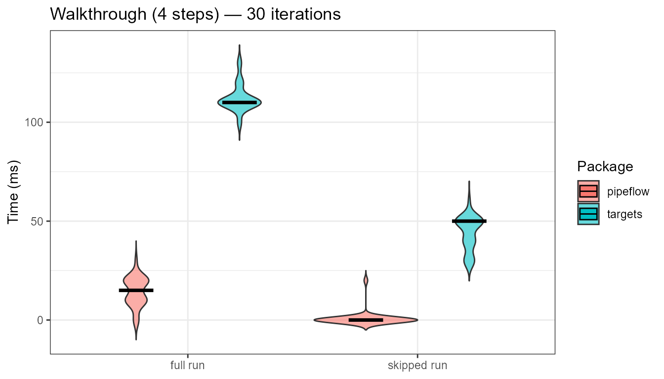
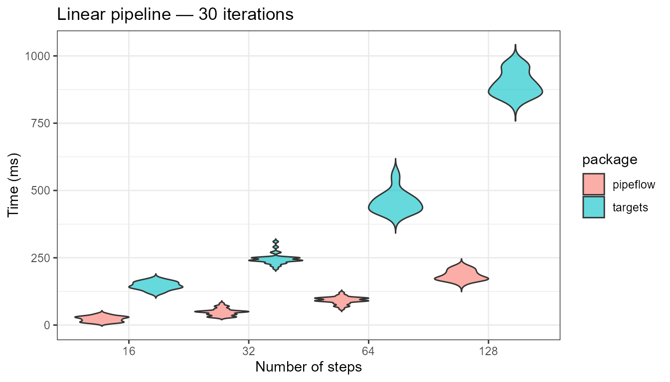
Long linear pipeline
Each step depends on the output of the previous step:
s0 -> s1 -> s2 -> ... -> sN. This measures the
overhead of managing the pipeline structure and skipping logic as the
number of steps increases. We benchmark at 16, 32, 64, and 128 steps to
show how the per-step cost scales.
pipeflow pipeline
create_linear_pip <- function(n) {
    pip <- pip_new("linear") |> pip_add("s0", \(init = 0) init)

    for (i in seq_len(n)) {
        pip_add(pip, step = paste0("s", i), \(x = ~ -1) x + 1)
    }
    pip
}

# Verify
p <- create_linear_pip(3)
pip_run(p)
# info [2026-06-20 19:21:23.552 UTC]: Start run of pipeflow_pip 'linear'
# info [2026-06-20 19:21:23.552 UTC]: Step 1/4 s0
# info [2026-06-20 19:21:23.553 UTC]: Step 2/4 s1
# info [2026-06-20 19:21:23.554 UTC]: Step 3/4 s2
# info [2026-06-20 19:21:23.556 UTC]: Step 4/4 s3
# info [2026-06-20 19:21:23.557 UTC]: Finished run of pipeflow_pip 'linear'
stopifnot(p[["s3", "out"]] == 3)
targets pipeline
create_linear_tar <- function(n) {
    init <- tar_target(s0, 0)
    rest <- lapply(
        seq_len(n),
        FUN = \(i) tar_target_raw(
            sprintf("s%d", i),
            call("+", as.symbol(sprintf("s%d", i - 1)), 1)
        )
    )
    c(list(init), rest)
}

# Verify
tar_dir({
    tar_script(create_linear_tar(3), ask = FALSE)
    tar_make_here(reporter = "timestamp")
    stopifnot(tar_read(s3) == 3)
})
# 2026-06-20 21:21:23.65 dispatched target s0
# 2026-06-20 21:21:23.66 completed target s0 [0ms, 49 B]
# 2026-06-20 21:21:23.66 dispatched target s1
# 2026-06-20 21:21:23.66 completed target s1 [0ms, 51 B]
# 2026-06-20 21:21:23.66 dispatched target s2
# 2026-06-20 21:21:23.67 completed target s2 [0ms, 50 B]
# 2026-06-20 21:21:23.67 dispatched target s3
# 2026-06-20 21:21:23.68 completed target s3 [0ms, 51 B]
# ✔ 2026-06-20 21:21:23.68 ended pipeline [61ms, 4 completed, 0 skipped]
# 
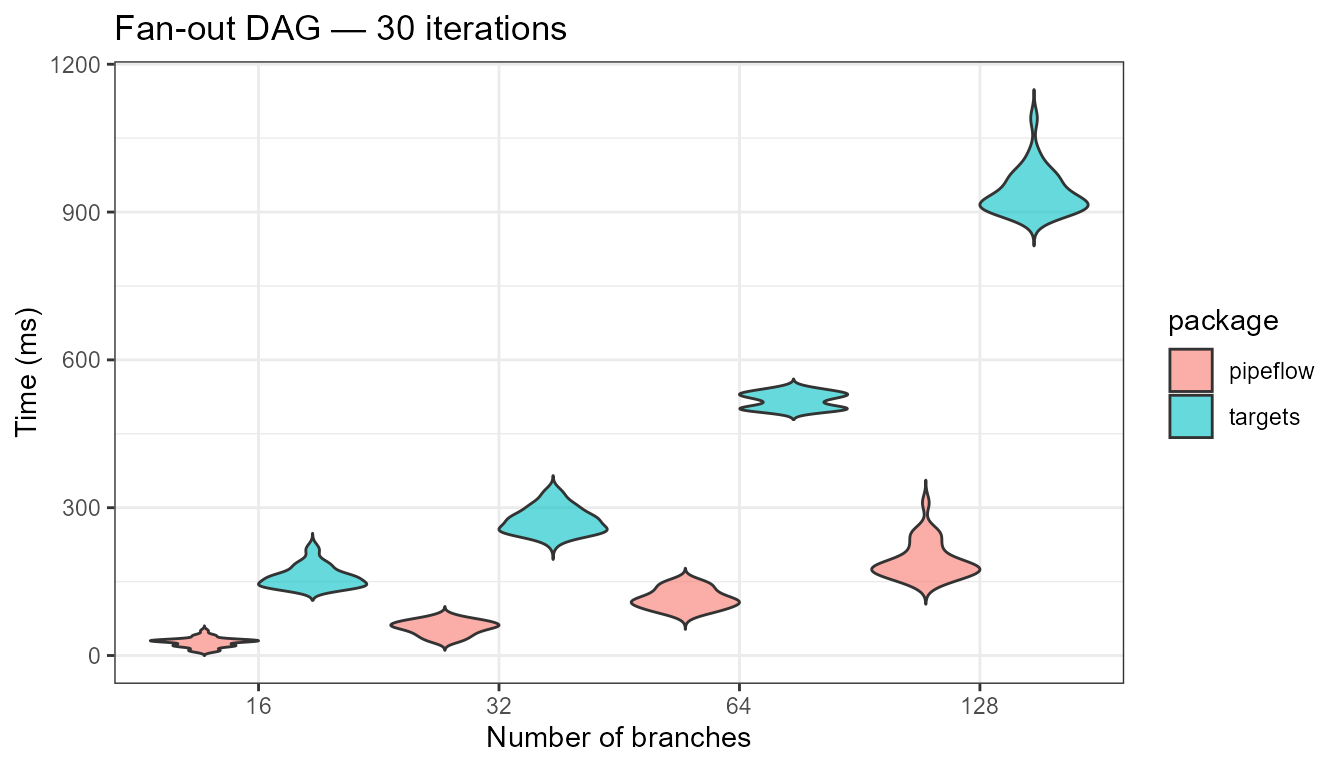
DAG with branching
A source feeds N parallel branches, all converging on a single sink step. This tests scalability with fan-out structures and how each package handles wide dependency graphs — from 16 up to 128 parallel branches. Unlike the linear pipeline, all branches can potentially run independently once the source completes.
dag_source <- function() 1
dag_branch <- function(x) x + 1
dag_sink   <- function(...) sum(...)
pipeflow pipeline
make_branch_pip <- function(n) {
    pip <- pip_new("dag") |> pip_add("source", dag_source)
    for (i in seq_len(n))
        pip_add(pip, paste0("b", i), \(x = ~source) dag_branch(x))

    sink_args <- paste(
        sprintf("x%s = ~b%s", seq_len(n), seq_len(n)),
        collapse = ", "
    )
    sink_call <- paste(paste0("x", seq_len(n)), collapse = ", ")
    eval(parse(text = sprintf(
        "pip_add(pip, 'sink', function(%s) { dag_sink(%s) })",
        sink_args, sink_call
    )))
    invisible(pip)
}

p4 <- make_branch_pip(4)
pip_run(p4)
# info [2026-06-20 19:22:29.081 UTC]: Start run of pipeflow_pip 'dag'
# info [2026-06-20 19:22:29.081 UTC]: Step 1/6 source
# info [2026-06-20 19:22:29.082 UTC]: Step 2/6 b1
# info [2026-06-20 19:22:29.084 UTC]: Step 3/6 b2
# info [2026-06-20 19:22:29.087 UTC]: Step 4/6 b3
# info [2026-06-20 19:22:29.089 UTC]: Step 5/6 b4
# info [2026-06-20 19:22:29.090 UTC]: Step 6/6 sink
# info [2026-06-20 19:22:29.092 UTC]: Finished run of pipeflow_pip 'dag'
stopifnot(p4[["sink", "out"]] == 8)
targets pipeline
make_branch_tar <- function(n) {
    source <- tar_target(source, dag_source())
    branches <- lapply(
        seq_len(n),
        FUN = \(i) tar_target_raw(
            sprintf("b%d", i),
            call("dag_branch", as.symbol("source"))
        )
    )
    sink <- tar_target_raw(
        "sink",
        as.call(c(
            as.symbol("dag_sink"),
            lapply(paste0("b", seq_len(n)), as.symbol)
        ))
    )
    c(list(source), branches, list(sink))
}

# Verify
tar_dir({
    tar_script(make_branch_tar(4), ask = FALSE)
    tar_make_here(reporter = "timestamp")
    stopifnot(tar_read(sink) == 8)
})
# 2026-06-20 21:22:29.19 dispatched target source
# 2026-06-20 21:22:29.19 completed target source [0ms, 51 B]
# 2026-06-20 21:22:29.20 dispatched target b1
# 2026-06-20 21:22:29.21 completed target b1 [0ms, 50 B]
# 2026-06-20 21:22:29.21 dispatched target b2
# 2026-06-20 21:22:29.21 completed target b2 [0ms, 50 B]
# 2026-06-20 21:22:29.22 dispatched target b3
# 2026-06-20 21:22:29.22 completed target b3 [0ms, 50 B]
# 2026-06-20 21:22:29.22 dispatched target b4
# 2026-06-20 21:22:29.23 completed target b4 [0ms, 50 B]
# 2026-06-20 21:22:29.23 dispatched target sink
# 2026-06-20 21:22:29.24 completed target sink [0ms, 51 B]
# ✔ 2026-06-20 21:22:29.24 ended pipeline [70ms, 6 completed, 0 skipped]
#